AI Canopy-to-Impervious Ratio: Intelligent Urban Planning

Executive Summary #
Client:
Baum Schwyz (University Project)
The Main Win: Built a full-stack web platform that fuses 3D LiDAR data with 2D aerial imagery to identify urban heat islands with ~85% segmentation accuracy. Users can draw regions on an interactive map and receive automated CIR analysis.
Tech Stack: PyTorch (U-Net), LiDAR Point Clouds, PostGIS, FastAPI, React, MapLibre GL, Docker.
The Challenge #
Context: The
Baum Schwyz collective aims to mitigate urban heat islands and biodiversity loss by increasing tree coverage in the Canton of Schwyz.
The Pain Point: Effective intervention requires knowing exactly where a new tree provides the most benefit. The existing approach relied on “gut feeling” or manual surveys, which are unscalable and subjective. High-resolution data on “impervious surfaces” (concrete/asphalt) was simply not available for the specific regions of interest.
Business Impact: Without precise data, resources risk being allocated inefficiently—planting trees in areas that are already green while missing critical heat hotspots (areas with high sealing and low canopy).
The Solution #
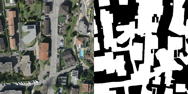
Strategy: I designed a multi-modal data fusion pipeline. Instead of training a model to find trees (which is visually complex), I leveraged existing high-precision LiDAR data for vegetation. I then focused my Machine Learning efforts on the missing piece: detecting sealed surfaces (roads, roofs, parking lots) from aerial imagery.
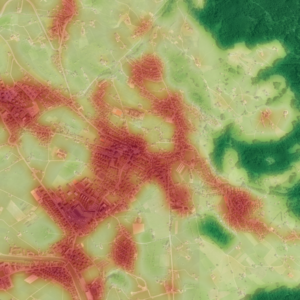
Key Feature: The Canopy-to-Impervious Ratio (CIR). This custom metric quantifies the relationship between shade and concrete per grid cell, generating a visual “Heatmap” for decision-makers.
Decision: I initially experimented with YOLO (Object Detection) but quickly pivoted. A road is not a discrete object like a “car” or “person” with a bounding box; it is a continuous, irregular surface. I switched to U-Net (Semantic Segmentation), which classifies every individual pixel, offering the granular precision needed for area calculations.

The Results #
- Accuracy: The custom U-Net model achieved an IoU (Intersection-over-Union) of ~85% on the validation set.
- Deliverables: The pipeline automatically generates:
- GIS Shapefiles (.shp): Compatible with official settlement data for technical planning.
- Visual Reports: Intuitive heatmaps that allow non-technical stakeholders to spot “red zones” (heat islands) instantly.
Technical Architecture #
Current Status: The Inference Pipeline #
The core logic currently operates as a Python script (cir_report) that processes specific geographic bounds:
- Input: User provides a Bounding Box (Swiss LV95 coordinates).
- Data Ingestion: Downloads RGB Aerial Imagery tiles (Swisstopo) and fetches 3D LiDAR point clouds.
- Processing:
- LiDAR Path: Filters point clouds for
class=vegetationandheight > 3m. - Vision Path: Tiles images (512x512), feeds them to U-Net for segmentation, and stitches masks.
- LiDAR Path: Filters point clouds for
- Fusion: Overlays datasets and applies Gaussian smoothing.
- Output: Exports GeoTIFFs, Shapefiles, and PNG reports.
Web Platform Architecture #
The tool is deployed as a hosted web application. Users request analyses via an interactive map interface—no local scripts required.
Key Platform Features:
- Interactive Map Interface: Draw bounding boxes on satellite/OSM basemaps to define analysis regions (max 4 km²).
- Vector Tile Serving: Dynamic MVT tiles for canopy/impervious polygons and CIR heatmap grid via
ST_AsMVT. - Spatial Optimization: GIST indexes on geometry columns +
ST_Subdivideduring INSERT (splits polygons to <255 vertices) for fast tile queries. - Tile Reuse: Worker caches processed LiDAR tiles by model version. Overlapping areas reuse existing canopy results.
- Export Options: Download results as PNG heatmap (with optional Swisstopo basemap) or GeoPackage/Shapefile.
Key Technical Challenges #
Challenge 1: “Is that a lake or a parking lot?” The model initially struggled to distinguish between dark, smooth water bodies and fresh asphalt. Conversely, compacted gravel paths looked identical to concrete.
The Fix: I implemented a strict labeling protocol (“Definitively Sealed” vs. “Definitively Not Sealed”) and conducted targeted “active learning” rounds. I specifically labeled edge cases like lakeshores and forest paths to force the model to learn the contextual differences.
Challenge 2: The Resolution limit Feeding a 2000x2000px aerial map into a standard CNN destroys the fine details needed to spot a narrow sidewalk.
The Fix: I implemented a tiling mechanism. The pipeline slices the geographic area into 512x512 training tiles (and 256x256 inference tiles). This allows the model to “see” small features without blowing up GPU memory.
Implementation Details #
The core of the solution is the inference loop that handles the tiling and stitching logic to ensure seamless maps.
def process_tile(model, tile: np.ndarray, device: str) -> np.ndarray:
    """
    Runs inference on a single image tile using the trained U-Net.

    Args:
        model: Loaded PyTorch U-Net model.
        tile: Numpy array of shape (H, W, C), normalized.
        device: 'cuda' or 'cpu'.

    Returns:
        Binary mask (H, W) where 1 indicates impervious surface.
    """
    # 1. Preprocess: (H, W, C) -> (1, C, H, W)
    input_tensor = torch.from_numpy(tile).permute(2, 0, 1).unsqueeze(0).float()
    input_tensor = input_tensor.to(device)

    # 2. Inference
    model.eval()
    with torch.no_grad():
        output = model(input_tensor)
        # Apply sigmoid to map logits to probabilities [0, 1]
        probs = torch.sigmoid(output)

    # 3. Postprocess: Thresholding at 0.5 for binary classification
    mask = (probs > 0.5).float().squeeze().cpu().numpy()

    return mask
Logic: The U-Net architecture uses a ResNet34 backbone pre-trained on ImageNet. This allows the model to understand basic features (edges, textures) immediately, reducing training time. I treated the problem as a binary segmentation task: Class 0 (Permeable/Nature) vs. Class 1 (Impervious/Artificial).
Infrastructure & Deployment #
- Containerization: Multi-stage Docker builds for all services (React frontend via nginx, FastAPI, Inference Worker).
- Job Queue: PostgreSQL-based queue using
SELECT FOR UPDATE SKIP LOCKED. Includes stale job recovery (30-min timeout). - Hosting: Linux VPS with Docker Compose orchestration. Resource limits: Worker 3GB, API 1GB, PostgreSQL 2GB.
- CI/CD: GitLab CI pipeline runs tests and deploys. Model artifacts stored in GitLab Package Registry.
